Components of a Transformer Architecture in LLMs

a concept first tour of how transformers work – Transformer Architecture

I’ve always been curious about what’s actually happening inside a transformer, not the API call, not the chat interface, but the actual mechanics underneath. How does attention “know” which words matter? What does a weight matrix encode meaning at all? This post is me pulling apart every component to answer those questions for myself, one piece at a time.

Transformer – Full Picture

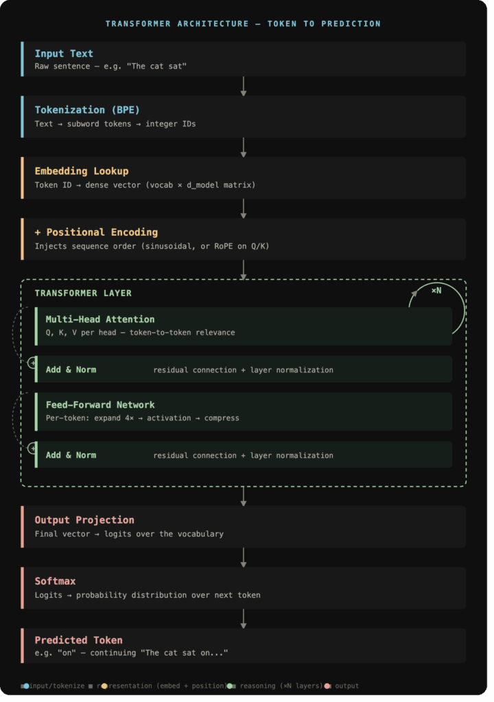
Before dividing each component, it helps to hold the whole pipeline in one view. A transformer takes a sequence of text, converts it into mathematical objects, and passes those objects through stack of reasoning layers, and outputs a probability distribution over what comes next. This very final step of predicting next token isn the only training objective. Everything else the model can do emerges from doing that one thing at enormous scale.

1. Tokenization

Raw text is split into tokens(subword chunks) and each is mapped to an integer ID. This is the first cost gate where everything is billed here. The number of token the input text chucked to is considered as input tokens per prompt

2. Embedding

Each token ID is looked up in a matrix to produce a dense vector. The model now works entirely in continuous vector space.

3. Positional Encoding

Position information is injected into each vector. Without this, the model has no sense of word order.

4. Transformer Layers (×N)

A stack of identical layers, each containing Multi-Head Attention and a Feed-Forward Network. This is where reasoning happens and where most compute lives.

5. Output Projection

The final vector is projected to vocabulary size and converted to probabilities. The highest-probability token is the prediction.

---

Component 01

Tokenization

A Transformer processes text in two directions, going in (mapping a token to a vector) and going out (mapping a hidden state back into a token vocabulary. We almost think that each word is considered as a token, which sometimes may be true but often times not in LLM world. To start with, text cannot enter a neural network directly. Tokenization acts as translation layer where strings of characters are broken down into much simpler pieces called tokens (words, characters, or subwords) which are then converted into integer IDs that a model can process.

Byte Pair Encoding

The dominant algorithm used for tokenization is Byte Pair Encoding (BPE). It starts with individual characters and iteratively merges the most frequently co-occurring pair into a single unit. After enough merges, typically 50,000 to 100,000 common words become single tokens, rare words get split into pieces, and novel words can still be represented as combinations of known subwords.

Tokenizer relies on vocab.json and merge.txt to produce tokens. vocab.json is a static lookup json where each token corresponds to a uniqueIDs which later gets used to find the latent vectors in Embedding matrix.

A merges.txt file is a plain text file. Each line contains exactly two tokens separated by a space.The order of the lines is critical as the top line is the highest priority rule, and the bottom line is the lowest priority rule.

BPE Merge Example

  Input:   "unbelievable"

  Start:   u · n · b · e · l · i · e · v · a · b · l · e
           (12 tokens)

  After merges:
           un · be · liev · able
           (4 tokens)

  Token IDs: [1842, 307, 2871, 481]
  

merge.txt

#version: 0.2
i n
in g
e a
l ea
lea r
lear n
Ġ l
Ġl earn

vocab.json
{
  "<s>": 0,
  "</s>": 1,
  "<unk>": 2,
  "<pad>": 3,
  "the": 4,
  "a": 5,
  "and": 6,
  "cat": 7,
  "dog": 8,
  "run": 9,
  "ing": 10,
  "ed": 11,
  "Ġlearn": 12,
  "Ġlearning": 13,
}

Special Tokens (IDs 0–3): These are structural markers for the model. For example, <s> marks the start of a sentence, and <unk> stands for “unknown” if a character cannot be tokenized.
Subwords (IDs 10–11): Fragments like ing and ed allow the model to build larger words (e.g., run + ing = running) without needing a separate ID for every single variation of a word.
The Ġ Symbol (IDs 12–13): In specific tokenizers, this special character represents a space before the word. This helps the model know where words begin and end.

Component 02

Embeddings – How it works

Any large language model typically contains two large matrices input embedding matrix and output project matrix, where each have a row or a column for every possible token in the vocabulary list.

The input embedding matrix converts token IDs into dense vectors at the start of the network. If the vocabulary has V words and the embedding dimension is d, this matrix has shape V×d. The output projection matrix converts the final hidden states back into a probability distribution over the vocabulary (the logits before softmax). This matrix typically has shape d×V, often the transpose of an embedding-like matrix.

After the tokenizer generates the sequence of token IDs, each ID retrieves a corresponding row from the embedding matrix. The result is a dense vector of floating point numbers, typically 768 to 12,288 numbers long depending on the model’s size. This vector is models internal representation of that token.

Embedding Matrix Size

The embedding matrix has dimensions vocab_size * hidden_dim . For a model with a 50,000 – token vocabulary and 4,096 dimensional embeddings results in roughly 200 million individual parameters(more precisely floating point numbers). The amount of memory that takes to host this single table would be around 410 MB if half precision¹ is used for representation of these floating points.

Weight Tying

Weight tying is a technique where the same embedding matrix is shared between the input embedding layer and the output projection layer (often called the softmax layer or language model head) in a neural network. This sharing is mathematically possible because both layers serve related semantic roles. While the input embeddings map word meanings into the model, the output projections measure the similarity between hidden states and vocabulary words. Consequently, when two words share semantic meaning, their tied representations ensure that their input embeddings are positioned closely in space and their output vectors produce similar logit² patterns.

Component 03

Positional Encoding

Transformers process all tokens in a sequence in parallel (unlike RNNs, which process tokens one at a time in order). This parallelism is central to its efficiency, but it introduces a limiting as self-attention on its own has no inherent notation of sequence of order. Self attention computes relationship between tokens based on their content or meaning not their position. So, without additional information on where each of the word of sentence is present, sentences with same set of words in a different order would be processed identically.

Positional encoding addresses this limitation by injecting information about each token’s position in the sequence into token’s numerical representation (token embeddings ), so that model can distinguish not only what a token is, but where it occurs relative to the rest of the sequence.

Positional encoding compliments word embedding

While token embeddings encode context-independent semantic features, they lack structural awareness, requiring explicit positional encodings to inject sequence order. For instance, the embedding for “dog” is identical whether “dog” is the first word or the last word of a sentence.

The original Transformer architecture (“Attention Is All You Need,” Vaswani et al., 2017)³ generates positional encodings using sine and cosine functions of varying frequency. For a position pos and a dimension index i, the formula is:

Here, d is the embedding dimension, and i ranges from 0 to d/2 - 1, since each value of i produces one sine value and one cosine value, together filling two of the d available dimensions. The term 10000 is a separately chosen constant that controls how widely the frequencies are spread across dimensions; it is not derived from d, but rather fixed by the original authors.

As i increases, the divisor 10000^(2i/d) grows larger, which slows the corresponding sine or cosine wave down. The practical effect is that low dimension indices oscillate rapidly as position increases, while high dimension indices oscillate very slowly. Reading across all dimensions at a fixed position produces a unique combination of values, a distinct “signature” for that position, similar to reading the angles of several clock hands spinning at different speeds at a single moment in time.

Sine and cosine are paired at each frequency, rather than using sine alone, for two reasons:

1. Disambiguation. The sine function is not one-to-one over a full oscillation, sin(x) and sin(π − x) can yield the same value, meaning two different positions could otherwise produce identical output on that dimension. Pairing sine with cosine, which together describe a point moving around a unit circle, removes this ambiguity.
2. Relative position computation. Standard trigonometric identities, such as sin(a + b) = sin(a)cos(b) + cos(a)sin(b), allow the positional encoding for position p + k to be expressed as a linear function of the encoding for position p. This gives the model a mathematically convenient way to represent relative distances between tokens, without needing that relationship to be explicitly labeled during training.

Conceptual Understanding of Positional Encoding – Example

Consider the sentence “The cat sat,” tokenized into three words at positions 0, 1, and 2. For clarity, assume a small embedding dimension of d = 4 (real transformer models typically use d = 512 or higher; the underlying computation is identical, simply repeated across more dimensions).

Step 1: Word embeddings. Assume the following (illustrative) learned embeddings:

Step 2: Positional encodings. With d = 4, i takes values 0 and 1, giving frequency divisors of 10000^0 = 1 and 10000^0.5 = 100. Applying the formula at each position:

Step 3: Combine embedding and positional encoding. Adding the two vectors element-wise for each word gives the final input passed into the transformer:

Each word now carries a representation that reflects both its meaning (from the embedding) and its position in the sentence (from the positional encoding). If the same word were to appear at a different position like for instance, if the sentence were “The cat sat, and the cat slept,” with “cat” appearing again later then its embedding component would remain the same, but its positional encoding would differ, producing a distinct final vector. This is the mechanism by which a transformer distinguishes between otherwise identical tokens based on where they occur in a sequence.

COMPONENT 04

Transformer Layers (xN)

Attention

Recurrent NN processes sequences step by step, compressing everything seen so far into a fixed-size hidden state. This creates couples of issues, information from early tokens degrades as the sequence gets longer, and computation is inherently sequential, which limits parallelization.

Attention addresses both. Instead of compressing history into a single vector, it allows a token to form a direct, weighted connection to any other token in the sequence, regardless of distance. It also parallelizes well, for instance an RNN⁴ must process token 2 before it can process token 3, because each step’s hidden state depends on the previous one. Attention has no such dependency.

Queries, Keys, and Values

Every input to an attention layer is a matrix of vectors, one row per token which already has embedding and positional encoding information.

• A query represents what a given token is “looking for.”
• A key represents what each token “offers” as a way of being matched against a query.
• A value represents the actual content that gets passed forward if a match is found.

Call this matrix X, with shape (n, d_model), where n is sequence length and d_model is the embedding dimension. From X, the model produces three derived representations using three learned weight matrices:

$W_Q$, $W_K$, and $W_V$ have shape $(d_{\text{model}} , \space d_k)$ (with V sometimes projected to a different dimension $d_v$, though in the original formulation $d_k = d_v$). The result is that Q, K, and V each have shape (n, $d_k$).Note that Q, K, and V all originate from the same input X in self-attention and the model isn’t retrieving from an external database, it is comparing tokens in a sequence to each other. This is what distinguishes self-attention from generic attention.

A Working Example

Extending the above example, the three vectors from“Example – Combining embeddings and positional encodings“ section to be called as stack X with shape (3, 4) are what the attention layer receives. Everything from here on operates on X, not on the embeddings and positional encodings separately; the two have already been fused.

Deriving Q, K, V

Three learned weight matrices project X into queries, keys, and values:

As with the embeddings or learned weight matrices with shape (d_model, d_k) , these are illustrative and in a real model they start as random initializations and are shaped entirely by training. In this example, (d_k = d_v = 4 = d_model), meaning the single attention head preserves the original embedding dimension. Real-world Transformer models extend this concept using multi-head attention, where the model dimension is split across multiple smaller attention heads, allowing the model to learn different representation patterns in parallel.

Multiplying each row of X by each matrix gives:

Multi Head Attention

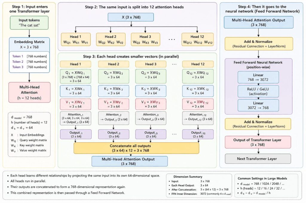
An attention head is a set of three learned matrices W_Q, W_K, W_V that creates Q, K, V from the same input embeddings. Each head learns a different way of looking at relationships between words.

When (d_model = 768) and there are (h = 12) attention heads, the model divides the embedding dimension by the number of heads (768 / 12 = 64). This allows the model to process tokens through 12 independent, smaller-dimensional subspaces, simultaneously learning diverse linguistic aspects like syntax, semantics, and grammar.

Attention scores – Q Kᵀ

Every query is compared against every key via a dot product, producing a 3×3 matrix which is one similarity score per pair of tokens:

Each row will become one token’s attention distribution, for instance row "The" says how much "The" resonates with each token (including itself), row "cat" says the same for "cat," and so on. Nothing has been normalized yet, these are raw, unbounded dot products, and their scale grows with vector magnitude, which is exactly the problem the next step corrects for. The attention score between two tokens is the dot product of their Q and K vectors, scaled and normalized through softmax.

Scale – Softmax – Weighted Sum

Divide every score by √d_k = √4 = 2, then apply softmax independently to each row so it becomes a probability distribution over “which tokens does this token attend to”:

Each token’s new representation is its row of attention weights multiplied against the V matrix which is a weighted blend of all three value vectors

For example, the output for “The” is 0.0568·v_The + 0.8596·v_cat + 0.0837·v_sat, i.e. mostly v_cat with small contributions from the other two — matching the 0.8596 weight it placed on “cat”. These three output vectors replace the original X for this layer.

Feed-Forward Network – FFN

After attention, each token’s representation passes independently through a small two-layer network: a linear expansion, a nonlinear activation, and a linear compression back. This is the Feed-Forward Network (FFN).

The FFN expands the hidden dimension by a factor of 4 before compressing it back. A 4,096-dimensional model has an FFN with an intermediate width of 16,384. This expansion-compression pattern creates a bottleneck that forces the network to learn sparse, selective representations and it is where the bulk of the model’s parameters live.

Attention vs FFN

Research into transformer internals has revealed a useful division of labor. Attention layers route information between tokens where they figure out which tokens are relevant to which(refer to above example). FFN layers store and retrieve factual associations where they function more like a lookup table that maps input patterns to known facts. This is why we can sometimes edit a model’s factual knowledge by modifying specific FFN weights without touching attention at all.

  token vector      →  [4096 dims]
        ↓
  Linear (expand)   →  [16384 dims]
        ↓
  Activation (GELU) →  nonlinearity applied
        ↓
  Linear (compress) →  [4096 dims]
        ↓
  + residual connection from before FFN
  

Residual Connections

Each sublayer in a Transformer, including the attention layer and the feed-forward network (FFN), adds its output to the original input through a residual connection before passing the result to the next layer. This allows information from earlier representations to be preserved while enabling each layer to learn additional transformations. The model does not need to rebuild the entire representation at every layer; instead, it can focus on modifying only the information that needs to change.

Without residual connections, training very deep networks becomes more difficult because gradients can become smaller as they move backward through many layers. Residual connections help maintain stronger gradient flow, making it possible to effectively train deep Transformer models with many layers.

Layer Normalization

After each residual addition, the values are shifted and scaled so they have zero mean and unit variance across the feature dimension. This prevents activations from exploding or collapsing during training, which becomes critical when stacking dozens of layers.

A single transformer layer is: attention → residual → norm → FFN → residual → norm. Models stack many of these. The number of layers is “depth.” The hidden dimension size is “width.” Both are levers that increase capacity.

COMPONENT 05

Output – Predicting the Next Token

After the final Transformer layer, each token has a contextual vector representation that contains information from the entire input sequence based on the attention mechanism. For next-token prediction tasks, the representation of the final token is typically used because it incorporates information from the preceding tokens and provides the context needed to estimate the next token.

This final vector is passed through a linear layer that maps it to the vocabulary size, which may contain 50,000 or more possible tokens. A softmax function then converts these output scores into probabilities. The model produces a probability value for each possible next token and selects or ranks tokens based on these probabilities.

  Context: "The cat sat"

  Output probabilities:
  "on"       →  0.762  ← model's prediction
  "down"     →  0.091
  "there"    →  0.034
  "quietly"  →  0.012
  ... (49,996 more tokens)
  

Temperature and Sampling

During inference, a temperature parameter is used to adjust the model’s output probability distribution before applying the softmax function. A lower temperature value increases the difference between token probabilities, making the model more likely to select the highest probability token. A higher temperature value produces a more balanced distribution, allowing less probable tokens to have a higher chance of being selected.

Temperature controls the level of randomness in token generation. It is applied only during inference and does not modify the model parameters or affect the training

Wrap Up

Understanding the architecture provides the foundation for exploring how Transformer models are trained and optimized. The next level involves understanding gradient flow, fine-tuning approaches, and alignment techniques such as RLHF⁵ and DPO⁶ that improve model behavior. These training strategies play a key role in building models that are both capable and aligned with desired objectives.

Glossary

1. What is a “Slot” Made Of ? A “slot” in AI language is a container for one single parameter (a 16-bit number, which takes up 2 bytes or 32-bit / Full precision, which takes up 4 bytes). ↩︎
2. Logits : Logits can be any real number ranging from -∞ to +∞. Because humans and downstream systems generally prefer interpretable percentages, logits are usually fed into an activation function, such as Softmax or Sigmoid, to transform them into a probability distribution.  ↩︎
3. https://arxiv.org/abs/1706.03762 ↩︎
4. RNN: Recurrent Neural Network ↩︎
5. RLHF (Reinforcement Learning from Human Feedback):
   RLHF is a training approach where human preferences are used to train a reward model, and the language model is then optimized to produce responses that receive higher rewards. It helps align model outputs with human expectations such as helpfulness, safety, and quality. ↩︎
6. DPO (Direct Preference Optimization):
   DPO is an alternative alignment method that directly trains the model using preferred and rejected responses without requiring a separate reward model or reinforcement learning step. It adjusts the model to increase the likelihood of preferred responses and reduce the likelihood of less preferred ones.
   ↩︎