Build Neural Network : Feedforward and Backpropagation with NumPy

Understanding the inner workings of Artificial Neural Network (NN) is crucial for anyone delving into the field of deep learning. This post will explore forward propagation, backward propagation, the critical role of weights and biases, and positive vs negative gradients.

Using Python libraries like PyTorch or TensorFlow makes building a neural network architecture seem straightforward—until you want to really understand how each neuron contributes to the learning process. Gaining this deep intuition can be challenging, especially as the network grows in size (trust me, it can get overwhelming even with the simplest!). To make it easier to grasp, I’ll break things down step by step with underlying matrices. And yes we will only use NumPy library!

---

Understanding Neural Network Layer Interactions

The core concept behind the large-scale processing of data in a Neural Network (NN) is based on the principle that each layer’s neurons utilize the activations (outputs) from the preceding layer as their inputs.

Building a 2-Layer Neural Network with NumPy

Let’s start with a simple example of a 2-layer neural network implemented in NumPy. This network consists of an input layer with 5 features, two hidden layers each with 10 neurons that use the ReLU¹ activation function, and an output layer with 4 neurons. The output layer employs the Softmax activation function², making it well-suited for multi-class classification tasks.

Forward Propagation: The Prediction Phase

Before going further into forward propagation, lets look at what are weights and biases of model, which often are referred to as model parameters.

Model Weight (w) :

A weight represents the strength or importance of the connection between two neurons in adjacent layers. Each weight is associated with an input feature and is used to scale the importance of that input to the output.

   

x – Input feature value
w – weight associated with the input x
b – bias term

The weight helps the network learn which features are most relevant in predicting the output. For instance, in a classification task, the weight could help the model recognize which aspects of the data are important for distinguishing between classes. Over time, during training, the weights are adjusted (via back propagation and gradient descent) to minimize the loss, leading to better predictions.

This transformation w⋅x scales the input, emphasizing or de-emphasizing different features depending on the magnitude of the weight. For example:

• Large weights: Inputs will have a larger impact on the output.
• Small weights: Inputs will have a smaller impact.

Model Bias (b) :

A bias is a parameter that allows the model to shift the activation function to the left or right. Biases are added to the weighted sum of inputs (before applying the activation function). The bias term shifts the activation function’s threshold, allowing the neuron to “fire” (produce a non-zero output) even when the input is entirely zero.

---

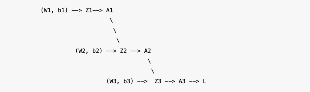
Forward Propagation :

Further breakdown of how matrices look like at every layer for Z(pre-activation), A(post-activation), W and b.

When initializing a neural network, the weights are typically set to random values at the start of the training process. This is a crucial part of the learning process. Here weights are Weights and Biases.

---

Backward propagation : Learning from Errors

In neural networks, the rate of change in weights, determined by gradients, directly affects the loss, which measures the difference between the predicted and actual outputs. During back propagation, the algorithm computes these gradients by differentiating the loss function with respect to each weight.

By adjusting the weights in the opposite direction of the gradient (gradient descent), the network minimizes the loss. This iterative process fine-tunes the weights, reducing errors in predictions over time. The magnitude of these weight updates is controlled by the learning rate, which balances the speed of convergence and the stability of the training process.

Chain Rule :

The chain rule is a key component of back propagation in neural networks, enabling the calculation of gradients for each layer. It allows us to compute the derivative of the loss function with respect to the weights by breaking down the overall derivative into a series of simpler derivatives.

Starting from the output layer, the chain rule is applied to propagate the error backward through each layer, multiplying the gradients of subsequent layers.

---

Positive Gradient Vs Negative Gradient

To understand the effect of positive gradient(slop or rate of change) or negative gradient on Loss function, lets take an example, if we do dL/dW the change is 0.5 vs -0.5 what does that value indicate ?

1. dL/dW = 0.5 : Rate of change in loss when we do a small change in weight (w) is +0.5
   • A positive gradient means that increasing the weight W will increase the loss L.
   • We have to move weights in the opposite direction of L, as the idea is to stay close to ground truth value which is Y
   • To reduce the loss, the weight should be decreased. This is why in gradient descent, the weight update formula subtracts the gradient multiplied by the learning rate.
   • A positive gradient means the weight needs to be decreased to reduce the loss.
2. dL/dW = -0.5 : Rate of change in loss when we do a small change in weight (w) is -0.5
   • A negative gradient indicates that increasing the weight W will decrease the loss L.
   • Negative Gradient (−0.5): This means that the loss decreases as the weight W increases. Therefore, increasing W will reduce the loss.
3. Magnitude of Gradient (e.g., 0.5 or -0.5)
   • The absolute value of gradient shows how steeply the loss changes w.r.t change in weight (w).
   • The larger magnitude represents more pronounced impact on the loss, implying a steeper slope, and hence a larger adjustment to the weight.Learning rate here plays a crucial role so the training process does not overshoot the local minima.
   • A smaller magnitude would suggest a more gradual change in loss, leading to smaller weight updates.s

---

Link to Github

Here is the link to my Github where there are more detailed notes at every step along with what I have on this blog post. Feel free to check.

2-LAYER-NN-NumPy

---

Wrapping Up: Forward and Backward Calculations with NumPy

To wrap up, in this post, we’ve explored the initial steps of forward and backward calculations in neural networks, using NumPy for hands-on calculations. These foundational operations are crucial for understanding how neural networks learn and adjust their weights during training. By manually computing these steps, we gain deeper insights into the inner workings of neural networks and the importance of operations like matrix multiplication and gradient computation. This knowledge lays the groundwork for tackling more complex challenges in neural network training, which we will dive into in future posts.

1. ReLU – Rectified Linear Unit. ReLU(x)=max(0,x) ↩︎
2. Softmax Activation :
   It converts raw scores (logits) from the network into probabilities by applying the exponential function and normalizing the output. The result is a vector of values between 0 and 1, which can be interpreted as probabilities that sum to 1. ↩︎