
Most engineers including myself may have met large language models through an API such as OpenAI’s GPT-4, Anthropic’s Claude, or Google’s Gemini. These are systems that process input tokens and return output tokens without exposing their internal mechanisms. In open-source LLMs, developers interact directly with tensors instead of relying on endpoint APIs.
This post walks through the mechanics of fine-tuning open-source large language models, explains why LoRA(Low-Rank Adaptation) exists, and shows mathematical and architecture context behind it.
Index
Open vs. Closed Model Architectures
Fine-Tuning Techniques in the Open Ecosystem
The Engineering Challenge: Updating Billions of Parameters
Understanding Low-Rank Decomposition in a Neural Network
LoRA Adapters and change in Inference
Fine Tuning Efficiency Comparison
Open vs. Closed Model Architectures
At first glance, GPT-4, Gemini 1.5 Pro, Claude 3, and LLaMA 3 all behave similarly where input prompt is given and an intelligent response is returned back. Under the hood, though, they belong to two very different worlds.
Large-language-model development has split largely into two clear ecosystems.
Closed systems : OpenAI’s GPT-series, Google’s Gemini, Anthropic’s Claude which are delivered as hosted APIs. These are products not artifacts.
Open-weight systems : LLaMA 3, Mistral 7B, Gemma 2, Qwen 2.5, Phi-3 which are released as downloadable artifacts that engineers can modify, extend, and redeploy. These are software components that can be engineered into systems.
The availability of weights transforms LLM work from API consumption to systems engineering. In essence closed models are services while open models are considered software asserts.
Closed Model Architecture
Open Model Architecture
Closed-model providers control the entire training and deployment stack.
Weights, tokenizers, and optimization processes remain proprietary.
Access is mediated through an API endpoint, providing simplicity and performance but little visibility or customization.
Open-source LLMs expose model definitions and checkpoint files.
Their weights can be cloned, quantized, instrumented, and fine-tuned under self-managed infrastructure.
This allows architectural experimentation, domain alignment, and compliance-controlled deployments.
The cost here is operational complexity, serving, updating, and aligning the model must be handled internally.
Fine-Tuning Techniques in the Open Ecosystem
Open source model has provision to download the weights. “Fine-tuning” in this context means adjusting the model to follow specific instructions, speak in a particular tone, or perform domain-specific reasoning. There’s a spectrum of techniques, from non-destructive to fully invasive.
There are several fine tuning techniques that can be employed on open model to adapt to domain specific tasks. Of which, most common are prompt engineering, prefix or Adapter Tuning, LoRA / QLoRA (Low-Rank Adaptation) and of course Full Fine-Tuning which is rarely done.
The Engineering Challenge: Updating Billions of Parameters – Full Fine Tuning
A LLaMA 3-8B model contains ~8 billion parameters distributed across transformer blocks. Each block has projection matrices, Wq, Wk, Wv, Wo for self-attention, plus feed-forward layers.
A full fine-tune means recomputing gradients and optimizer states for every one of those numbers. On A100s, that’s multiple GPUs running for days. It is rarely needed. The base model already knows grammar, code syntax, and reasoning. For fine tuning the necessity is to adjust how it applies that knowledge for domain specific tasks.
The LoRA Idea: Low-Rank Adaptation
A modern LLM is a stack of transformer blocks, each full of dense matrices often with tens of billions of parameters which are already optimized to predict the next token over a vast corpus.
Fine-tuning large language models (LLMs) such as LLaMA, Falcon, or Mistral often involves
- Hundreds of GBs of GPU memory,
- High network bandwidth for parameter synchronization, and
- Large checkpoint storage (tens of GBs per variant).
Yet in practice, most downstream tasks require adapting only a small subspace of the model’s latent space1, e.g., tuning language tone or factual grounding. Also Re-training every parameter is rarely done outside major labs because it demands multi-GPU clusters and precise optimization tricks (mixed precision, gradient checkpointing, learning-rate schedulers). Full fine-tuning only needed to re-learn the language distribution, say, for a new language or completely different domain like genomics.
LoRA (Low-Rank Adaptation), introduced by Hu et al. (2021), is a technique that enables parameter-efficient fine-tuning(PEFT) by updating only a small number of additional matrices(low rank) rather than modifying the full weight tensors of the model. This approach achieves near full fine-tuning performance while drastically reducing computational and storage costs.
The Core Idea – Low-Rank Decomposition
Rank : A matrix’s rank is the number of independent rows or columns it has or essentially how much unique information it contains.
If W0 is a dxk matrix then its maximum rank is min(d,k)



Every weight matrix in a neural network (say, in a Transformer) encodes learned relationships between input and output dimensions. For example, a linear layer might have a weight matrix


In large language models (LLMs), these matrices can be huge with millions of parameters each.
But research has shown that the changes introduced by fine-tuning (the difference between the pre-trained weight W0 and the fine-tuned weight W) often lie in a low-dimensional subspace.
This means the “update” matrix ΔW = W−W0 does not need full rank ( it doesn’t need as many degrees of freedom as W0 itself). It is this observation that is the foundation for Low-Rank Decomposition.
Example: Understanding Low-Rank Decomposition in a Neural Network
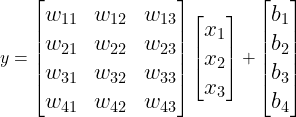
Step 1 : A Fully Connected layer (linear layer) in neural network

- x is the input vector (say, 3-dimensional),
- 4×3 weight matrix,
- y is the 4-dimensional output.
Example base (pre-trained) weight looks like
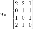
2. Fine-Tuning Normally (Full-Rank Update)
When a model is fully fine tuned it adjusts or nudges the final weights in such a way that inference becomes better. Let’s say fine-tuning yields a small change ΔW.
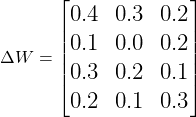
That’s 12 new parameters to learn.And the full fine-tuned weights would look like

So far, this is standard full fine-tuning where every parameter is updated.
3. Introducing Low-Rank Decomposition
Instead of directly learning ΔW (4×3 = 12 values), LoRA approximates it using two smaller matrices A and B
If a low rank of r = 2 is chosen then,

3.1 Example Matrices
Lets say LoRA learns:
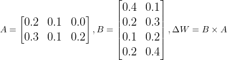
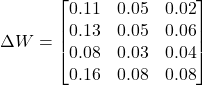
The LoRA ΔW isn’t identical, but it approximates the direction of change, enough for downstream tasks to perform similarly.
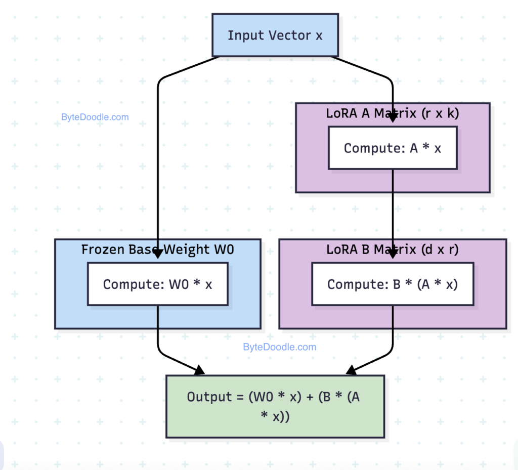
LoRA path (A → B) contains small trainable matrices that represents the low-rank fine tuning update
This shows LoRA as a residual low-rank update added on top of the pre-trained layer.
In a standard Transformer, layers like Linear / Dense projections such as the Query, Key, Value, and Output projections in self-attention, contain large weight matrices W0
LoRA does not replace these matrices. It adds a small, trainable low-rank update in parallel to them.
LoRA Adapters and change in Inference
During inference, LoRA changes how the model transforms inputs by adding a learned correction to the output of certain layers, especially attention projections. LoRA changes the direction of the output vector by adding a small adapter vector that nudges the output towards something more appropriate for fine tuned task. LoRA gently steers the layer’s output without rewriting the original weights. Conceptually, LoRA makes the model pay attention to different things than before.
In a transformer when LoRA is applied to
q_proj(queries) leads to different attention patternsk_proj(keys) leads to different token importancev_proj(values) leads to different contextual reasoning

LoRA lives inside the linear projections. LoRA adapters simply augment specific projections, changing how attention and MLP2 layers behave, without altering the base weights.
q_proj,k_proj,v_proj, and ofteno_proj,up_proj,down_proj.- Each is conceptually:
W * x + LoRA(x)whereLoRA(x) = B(Ax).
Fine Tuning Efficiency Comparison
Full Fine tuning
- For larger matrices O(d×k)
- Memory compute is high in full fine tuning
- large layers (like 4096×4096), the difference is dramatic. Full fine-tune results in 16,777,216 parameters
LoRA
- For larger matrices O(r(d+k))
- Its much lower when using LoRA
- LoRA (r=8) then 65,536 parameters, almost 256× reduction
How to Decide the “Rank”
In order to answer the question of “how low rank has to be ?” there are several practical and empirical guidelines.
- Task complexity: Simpler classification or instruction-following tasks → smaller r (4–8).
Complex domain adaptation (code, math, reasoning) → higher r (16–64). - Model size: Larger models can often use smaller ranks because their base representations are already richer.
- Available compute: Higher rank increases both memory and compute linearly.
| Model | Typical r | Notes |
|---|---|---|
| 7B (LLaMA, Mistral) | 8–16 | Sweet spot for domain fine-tuning |
| 13B–30B | 4–8 | Larger capacity allows lower rank |
| 70B+ | 4 | PEFT baseline for large-scale adaptation |
Advantages of LoRA
Even if LoRA did not reduce the total number of parameters, it would still offer clear architectural and operational advantages.
- The pre-trained base weights W0 remain frozen, training becomes more stable and less prone to catastrophic forgetting.
- LoRA’s design is inherently modular as its adapter layers can be stored, loaded, or swapped independently, allowing the same base model to support multiple domain-specific variants without retraining.
- Training is faster since only a small set of adapter parameters participate in gradient computation, reducing synchronization overhead in distributed settings. This also translates to lower VRAM usage, as optimizer states and gradients are limited to a fraction of the model. Finally, LoRA enables composable fine-tuning, where multiple adapters (for example, legal and financial domains) can be layered or combined to create specialized capabilities with minimal additional cost.
Structural and Technical Limitations
- Low-rank constraint can be too restrictive
LoRA assumes the required update matrix is low-rank. This works for subtle behavioral changes but underperforms when deep architectural or semantic changes are needed, causing slow convergence or under fitting. - Overfitting on very small datasets
With tiny or noisy datasets, LoRA adapters can overfit quickly because the model expresses all adaptation within a narrow subspace. - Activation memory remains unchanged
LoRA reduces trainable parameters, but does not reduce activation memory, so GPU memory savings are limited unless paired with quantization (e.g., QLoRA). - Degradation under heavy distribution shift
When moving from general text to highly technical/legal/medical domains, LoRA may fail to capture the full shift unless rank is increased significantly, and adapters are added to MLP layers in addition to attention.
Avoid using LoRA for tasks that require high-rank transformations or broad capability changes, such as the introduction of new reasoning behaviors. LoRA may also be unsuitable when available datasets are extremely small or noisy, and where generalization is more important than rapid fitting. Additionally, scenarios that require full backbone plasticity, such as deep skill development or substantial model repurposing, are better served by full fine-tuning approaches.
Summary and Future Work
LoRA fine-tuning provides a disciplined mechanism for adapting open-source language models. LoRA changes inference by adding small, learned adjustments to the outputs of certain linear layers while keeping the original pre-trained weights frozen. These low-rank adapters gently steer the model’s internal representations toward the fine-tuned task without overwriting existing knowledge. As a result, the model attends differently, emphasizes different features, and produces domain-specialized behavior. In essence, LoRA subtly shifts the model’s computations to incorporate new skills while preserving its base capabilities.
By training a small number of low-rank parameters, practitioners can introduce new behaviors and domain expertise at minimal computational cost while preserving the pre-trained model’s general reasoning abilities.
This article is the first in a multi-part series; upcoming sections will explore dataset construction, evaluation strategies, and deployment patterns for production-grade fine-tuned models.
Further Reading (recent research)
PiSSA: Principal Subspace Initialization for LoRA — improves convergence by initializing adapters via SVD of the base weight matrix.
https://arxiv.org/abs/2404.02948
LoRA-FA: Memory-Efficient Low-Rank Adaptation — reduces memory footprint and improves stability for smaller GPUs.
https://arxiv.org/abs/2308.03303
GLoRA: Generalized Low-Rank Adaptation — extends LoRA to a larger set of model parameters and activations.
https://arxiv.org/abs/2306.07967
QLoRA: Efficient Finetuning of Quantized LLMs — combines 4-bit quantization with LoRA for extreme memory savings.
https://arxiv.org/abs/2305.14314
- Latent space: Latent space is a compressed, lower-dimensional representation of complex data that captures its essential features. More info on https://blog.bytedoodle.com/latent-factors-the-hidden-structure/ ↩︎
- MLP : MLP stands for Multilayer perceptron. MLP (Feed-Forward Network) in a Transformer is a two-layer neural network applied after attention. It expands the hidden dimension to a larger size, applies a non-linear activation (like GELU), and then projects it back down.
Its purpose is to help the model transform and refine the attended information. ↩︎